Trading Systems
Trading System Development – Part 1
I assume you know programming (maybe you are even a professional developer) and you have that trading itch. You probably have been trading manually with your broker here and there, but decided to step up your game and introduce computers into the equation to remove human emotions from your trading. However you don’t really know how to start. If that’s your case – rest assured, by the end of this article you should know how to explore your trading ideas to find the ones that work for you.
This article is written by a professional software developer with no distinct financial education and assumes the reader has a similar background. I will not be explaining programming related concepts in it. Also, there are an infinite number of ways to achieve the same goal, this article presents just one of them.
Lifecycle of a Trading Idea
Dear reader, you are in for an adventure you probably have never experienced as the way from “that excellent idea” you have to live deployment of algorithms is long and it will test a wide range of your skills from several different fields. Let’s discuss how we are doing this in UWS
Life cycle of trading ideas:
- Come up with an interesting idea (i.e. Moving Average crossover for Bitcoin)
- Get historical data for relevant asset (i.e. Bitcoin 5 minute intervals)
- Do vectorized backtest to quickly assess if your idea makes sense
- Do event based backtest to confirm conclusions from vectorized backtest
- Implement and integrate with broker API
- Deploy against demo account and observe results
- Deploy against live account
In this article I will focus on getting a trading idea and validating it against historic data (points from 1 to 4). In part 2 you can read about putting strategy into code integrating with broker API.
Get an idea
This is both easy and hard part. You probably have at least one in mind. You heard something on your favorite podcast or read it on some site or even just it appeared in your mind spontanously. That was the easy part – what is hard is to get the right idea. \<insert some trading idea references>
Get the data
Internet is full of data, free and paid. In our article we will use Stooq’s data (https://stooq.pl/db/), which is free of charge and formatted in a way that we will have to do some transformations as training exercise. Please be aware that Stooq imposes download limits and it is easy to get yourself locked out for a day. Be considerate aboutyour downloads.
Validate your concept
We have the idea and we have the data. We want to validate it to make sure we move to
Python Data Science tech stack
“Data Science? This is supposed to be about trading” I hear you say. Yes, my dear reader, Data Science tech stack brings us a lot of very useful tools for quickly validating or dismissing ideas. Let’s discuss them in details:
- Python – if you know any other programming language you can learn it in a blink of an eye and yet Python brings to the table a number of excellent libraries for working with data.
- NumPy – very fast library for multidimensional arrays, industry standard and base for number of other libraries
- Pandas – if you think data you should also think Pandas. It’s defacto industry starndard for data science, useful for holding, tranforming, querying etc. You can think about it as convenience wrapper of your NumPy arrays.
- Matplotlib – charting library, seamlessly integrated with Pandas. Also serves as base for other libraries, for example seaborn.
- SciPy – NumPy based library that adds more advanced operations (linear algebra, signal analysis, etc). We won’t be using it in this tutorial
- Scikit-Learn – for Machine Learning/Data Mining. We won’t be using it too.
- Jupyter Notebook – web application that allows you to write and execute python code, mix it together with markdown for very elegant and descriptive articles. Extension of Jupyter Notebook is Jupyter Lab, which gives you more IDE like user experience giving you additionally filesystem explorer, terminal window, etc. This article is written in Jupyter Lab.
For package manager we use Miniconda and/or pip. Sometimes packages are not avaialble in one or another, but they both integrate with each other pretty well.
Prepare your data with Pandas
First of all, let’s look at the downloaded data. This is how two first lines can look like.
<TICKER>,<PER>,<DATE>,<TIME>,<OPEN>,<HIGH>,<LOW>,<CLOSE>,<VOL>,<OPENINT>
^AEX,5,20210303,090500,667.6,668.19,667.5,667.76,0,0
We can see that first line defines columns, and data is separated by comma. This is very common case and we can use Pandas to read it:In [1]:
import pandas as pd
data = pd.read_csv('data_5.txt')
data
Out[1]:
| <TICKER> | <PER> | <DATE> | <TIME> | <OPEN> | <HIGH> | <LOW> | <CLOSE> | <VOL> | <OPENINT> | |
|---|---|---|---|---|---|---|---|---|---|---|
| 0 | ^AEX | 5 | 20210303 | 90500 | 667.60 | 668.19 | 667.50 | 667.76 | 0 | 0 |
| 1 | ^AEX | 5 | 20210303 | 91000 | 667.77 | 668.32 | 667.54 | 668.32 | 0 | 0 |
| 2 | ^AEX | 5 | 20210303 | 91500 | 668.30 | 668.62 | 668.26 | 668.26 | 0 | 0 |
| 3 | ^AEX | 5 | 20210303 | 92000 | 668.17 | 668.67 | 668.07 | 668.41 | 0 | 0 |
| 4 | ^AEX | 5 | 20210303 | 92500 | 668.25 | 668.42 | 667.92 | 668.13 | 0 | 0 |
| … | … | … | … | … | … | … | … | … | … | … |
| 719995 | XAUUSD | 5 | 20210330 | 224000 | 1683.36 | 1683.55 | 1682.81 | 1683.34 | 0 | 0 |
| 719996 | XAUUSD | 5 | 20210330 | 224500 | 1683.33 | 1684.37 | 1682.88 | 1684.30 | 0 | 0 |
| 719997 | XAUUSD | 5 | 20210330 | 225000 | 1684.31 | 1684.65 | 1683.71 | 1684.31 | 0 | 0 |
| 719998 | XAUUSD | 5 | 20210330 | 225500 | 1684.32 | 1685.02 | 1683.91 | 1684.97 | 0 | 0 |
| 719999 | XAUUSD | 5 | 20210330 | 230000 | 1684.99 | 1685.38 | 1684.46 | 1685.19 | 0 | 0 |
720000 rows × 10 columns
You can see two things straight away. First that Pandas has read 720000 rows and 10 columns and second that Jupyter Notebook displayed it for you in a very nice way.
For the purpose of this article we want only OHLC prices (open, high, low close) and timestamp and for just one asset, so we need to do some transformations. If you are coming from programming field, the way we are going to do this transformation may seem a bit awkward for you at the beginning, as it was for me. I was used to looping over data and performing various operations within. This however is not “pandas way”. How you can best utilize pandas is to perform vectorized operations.
Let’s take columns <DATE> and <TIME>. You can see that date is formatted in YYYYMMDD format, but time is either HmmSS or HHmmSS. leading zero is removed by Pandas, because it thinks both columns are numbers (and we know they are strings). Let’s fix that:In [2]:
data['<DATE>'] = data['<DATE>'].astype(str)
data['<TIME>'] = data['<TIME>'].apply(lambda x: str(x).zfill(6))
data
Out[2]:
| <TICKER> | <PER> | <DATE> | <TIME> | <OPEN> | <HIGH> | <LOW> | <CLOSE> | <VOL> | <OPENINT> | |
|---|---|---|---|---|---|---|---|---|---|---|
| 0 | ^AEX | 5 | 20210303 | 090500 | 667.60 | 668.19 | 667.50 | 667.76 | 0 | 0 |
| 1 | ^AEX | 5 | 20210303 | 091000 | 667.77 | 668.32 | 667.54 | 668.32 | 0 | 0 |
| 2 | ^AEX | 5 | 20210303 | 091500 | 668.30 | 668.62 | 668.26 | 668.26 | 0 | 0 |
| 3 | ^AEX | 5 | 20210303 | 092000 | 668.17 | 668.67 | 668.07 | 668.41 | 0 | 0 |
| 4 | ^AEX | 5 | 20210303 | 092500 | 668.25 | 668.42 | 667.92 | 668.13 | 0 | 0 |
| … | … | … | … | … | … | … | … | … | … | … |
| 719995 | XAUUSD | 5 | 20210330 | 224000 | 1683.36 | 1683.55 | 1682.81 | 1683.34 | 0 | 0 |
| 719996 | XAUUSD | 5 | 20210330 | 224500 | 1683.33 | 1684.37 | 1682.88 | 1684.30 | 0 | 0 |
| 719997 | XAUUSD | 5 | 20210330 | 225000 | 1684.31 | 1684.65 | 1683.71 | 1684.31 | 0 | 0 |
| 719998 | XAUUSD | 5 | 20210330 | 225500 | 1684.32 | 1685.02 | 1683.91 | 1684.97 | 0 | 0 |
| 719999 | XAUUSD | 5 | 20210330 | 230000 | 1684.99 | 1685.38 | 1684.46 | 1685.19 | 0 | 0 |
720000 rows × 10 columns
Let’s do bit of explanation here. First line tells pandas to set column <DATA> to content of column <DATA> but converted to string. Second line sets column <TIME> to be result of applying lambda to that column. You can see that we have now 090500 instead of 90500.
Now let’s merge these columns together and provide new column – timestamp:In [3]:
data['timestamp'] = pd.to_datetime(data['<DATE>'] + 'T' + data['<TIME>'])
data
Out[3]:
| <TICKER> | <PER> | <DATE> | <TIME> | <OPEN> | <HIGH> | <LOW> | <CLOSE> | <VOL> | <OPENINT> | timestamp | |
|---|---|---|---|---|---|---|---|---|---|---|---|
| 0 | ^AEX | 5 | 20210303 | 090500 | 667.60 | 668.19 | 667.50 | 667.76 | 0 | 0 | 2021-03-03 09:05:00 |
| 1 | ^AEX | 5 | 20210303 | 091000 | 667.77 | 668.32 | 667.54 | 668.32 | 0 | 0 | 2021-03-03 09:10:00 |
| 2 | ^AEX | 5 | 20210303 | 091500 | 668.30 | 668.62 | 668.26 | 668.26 | 0 | 0 | 2021-03-03 09:15:00 |
| 3 | ^AEX | 5 | 20210303 | 092000 | 668.17 | 668.67 | 668.07 | 668.41 | 0 | 0 | 2021-03-03 09:20:00 |
| 4 | ^AEX | 5 | 20210303 | 092500 | 668.25 | 668.42 | 667.92 | 668.13 | 0 | 0 | 2021-03-03 09:25:00 |
| … | … | … | … | … | … | … | … | … | … | … | … |
| 719995 | XAUUSD | 5 | 20210330 | 224000 | 1683.36 | 1683.55 | 1682.81 | 1683.34 | 0 | 0 | 2021-03-30 22:40:00 |
| 719996 | XAUUSD | 5 | 20210330 | 224500 | 1683.33 | 1684.37 | 1682.88 | 1684.30 | 0 | 0 | 2021-03-30 22:45:00 |
| 719997 | XAUUSD | 5 | 20210330 | 225000 | 1684.31 | 1684.65 | 1683.71 | 1684.31 | 0 | 0 | 2021-03-30 22:50:00 |
| 719998 | XAUUSD | 5 | 20210330 | 225500 | 1684.32 | 1685.02 | 1683.91 | 1684.97 | 0 | 0 | 2021-03-30 22:55:00 |
| 719999 | XAUUSD | 5 | 20210330 | 230000 | 1684.99 | 1685.38 | 1684.46 | 1685.19 | 0 | 0 | 2021-03-30 23:00:00 |
720000 rows × 11 columns
As you can see we have new column that holds timestamp as result of concatenating date and time columns. Sometimes you may need to provide date format to to_datetime function, but our case was straightforward enough that it was able to handle it without explicit format.
Let’s see how many different assets we have in downloaded data set and how many different time framesIn [4]:
assets = data['<TICKER>'].unique()
timeframes = data['<PER>'].unique()
print(f'There is {len(assets)} asset(s) in this data set: {assets}')
print(f'There is {len(timeframes)} timeframe(s) in this data set: {timeframes}')
There is 184 asset(s) in this data set: ['^AEX' '^AOR' '^ATH' '^BEL20' '^BET' '^BUX' '^BVP' '^CAC' '^CDAX' '^CRY'
 '^DAX' '^DJC' '^DJI' '^DJT' '^DJU' '^FMIB' '^FTM' '^HEX' '^HSI' '^IBEX'
 '^ICEX' '^IPC' '^IPSA' '^JCI' '^KLCI' '^KOSPI' '^MDAX' '^MOEX' '^MRV'
 '^MT30' '^NDQ' '^NDX' '^NKX' '^NOMUC' '^NZ50' '^OMXR' '^OMXS' '^OMXT'
 '^OMXV' '^OSEAX' '^PSEI' '^PSI20' '^PX' '^RTS' '^SAX' '^SDXP' '^SET'
 '^SHBS' '^SHC' '^SMI' '^SNX' '^SPX' '^STI' '^TASI' '^TDXP' '^TSX' '^TWSE'
 '^UKX' '^UX' '^XU100' '^SOFIX' 'A6.F' 'B6.F' 'CB.F' 'CC.F' 'CL.F'
 'CLCHF.F' 'CLEUR.F' 'CLPLN.F' 'CT.F' 'D6.F' 'DX.F' 'DY.F' 'E6.F' 'ES.F'
 'FBUX.F' 'FHSI.F' 'FSMI.F' 'FX.F' 'G.F' 'GC.F' 'GCCHF.F' 'GCEUR.F'
 'GCPLN.F' 'GG.F' 'HG.F' 'HGCHF.F' 'HGEUR.F' 'HGPLN.F' 'HO.F' 'HR.F'
 'J6.F' 'JGB.F' 'KC.F' 'LF.F' 'MX.F' 'NG.F' 'NQ.F' 'NY.F' 'OJ.F' 'PA.F'
 'PL.F' 'RJ.F' 'S6.F' 'SB.F' 'SI.F' 'SICHF.F' 'SIEUR.F' 'SIPLN.F' 'X.F'
 'YM.F' 'ZB.F' 'ZC.F' 'ZF.F' 'ZL.F' 'ZN.F' 'ZS.F' 'ZW.F' 'AUDCAD' 'AUDCHF'
 'AUDEUR' 'AUDGBP' 'AUDJPY' 'AUDPLN' 'AUDUSD' 'CADAUD' 'CADCHF' 'CADEUR'
 'CADGBP' 'CADJPY' 'CADPLN' 'CADUSD' 'CHFAUD' 'CHFCAD' 'CHFEUR' 'CHFGBP'
 'CHFJPY' 'CHFPLN' 'CHFUSD' 'EURAUD' 'EURCAD' 'EURCHF' 'EURGBP' 'EURJPY'
 'EURPLN' 'EURUSD' 'GBPAUD' 'GBPCAD' 'GBPCHF' 'GBPEUR' 'GBPJPY' 'GBPPLN'
 'GBPUSD' 'JPYAUD' 'JPYCAD' 'JPYCHF' 'JPYEUR' 'JPYGBP' 'JPYPLN' 'JPYUSD'
 'NZDUSD' 'USDAUD' 'USDCAD' 'USDCHF' 'USDEUR' 'USDGBP' 'USDJPY' 'USDPLN'
 'XAGAUD' 'XAGCAD' 'XAGCHF' 'XAGEUR' 'XAGGBP' 'XAGJPY' 'XAGPLN' 'XAGUSD'
 'XAUAUD' 'XAUCAD' 'XAUCHF' 'XAUEUR' 'XAUGBP' 'XAUJPY' 'XAUPLN' 'XAUUSD']
There is 1 timeframe(s) in this data set: [5]
In our downloaded set we have data for 18 different assets in 1 timeframe. For the purose of article we will pick gold against USD (XAUUSD).
Let’s prepare dataframe will will work onIn [5]:
data.index = data['timestamp']
df = data.loc[data['<TICKER>'] == 'XAUUSD'].copy().iloc[-200:]
df.drop(columns=['<PER>', '<TICKER>', '<VOL>', '<OPENINT>', '<DATE>', '<TIME>', 'timestamp'], inplace=True)
df.columns = ['o', 'h', 'l', 'c']
df
Out[5]:
| o | h | l | c | |
|---|---|---|---|---|
| timestamp | ||||
| 2021-03-30 06:25:00 | 1706.65 | 1707.21 | 1706.56 | 1707.09 |
| 2021-03-30 06:30:00 | 1707.08 | 1707.14 | 1706.69 | 1706.89 |
| 2021-03-30 06:35:00 | 1707.02 | 1707.13 | 1706.30 | 1706.50 |
| 2021-03-30 06:40:00 | 1706.50 | 1707.57 | 1706.47 | 1707.36 |
| 2021-03-30 06:45:00 | 1707.32 | 1707.75 | 1707.07 | 1707.43 |
| … | … | … | … | … |
| 2021-03-30 22:40:00 | 1683.36 | 1683.55 | 1682.81 | 1683.34 |
| 2021-03-30 22:45:00 | 1683.33 | 1684.37 | 1682.88 | 1684.30 |
| 2021-03-30 22:50:00 | 1684.31 | 1684.65 | 1683.71 | 1684.31 |
| 2021-03-30 22:55:00 | 1684.32 | 1685.02 | 1683.91 | 1684.97 |
| 2021-03-30 23:00:00 | 1684.99 | 1685.38 | 1684.46 | 1685.19 |
200 rows × 4 columns
First of all we index our dataframe by timestamp. Then we select and copy all rows that have ‘XAUUSD’ in <TICKER> and drop unnecessary columns (we took only last 200 data points not to clutter the chart via .iloc[-200] call) Dataframe operations are immutable by default, so either you have to assign results to new variable or add inplace=True. Lastly we rename columns.
Add technical indicators
In our strategy we will use Moving Average (20) and look for crossover points. First we need to calculate Moving Average and add it to our dataframe. We can use pandas built in fucntions or TA-lib for that (link). I’ll show both ways, you will see they are equivalentIn [6]:
import talib as ta

df['MA20'] = df['c'].rolling(20).mean()
df['SMA20'] = ta.SMA(df['c'], 20)
display(df)
| o | h | l | c | MA20 | SMA20 | |
|---|---|---|---|---|---|---|
| timestamp | ||||||
| 2021-03-30 06:25:00 | 1706.65 | 1707.21 | 1706.56 | 1707.09 | NaN | NaN |
| 2021-03-30 06:30:00 | 1707.08 | 1707.14 | 1706.69 | 1706.89 | NaN | NaN |
| 2021-03-30 06:35:00 | 1707.02 | 1707.13 | 1706.30 | 1706.50 | NaN | NaN |
| 2021-03-30 06:40:00 | 1706.50 | 1707.57 | 1706.47 | 1707.36 | NaN | NaN |
| 2021-03-30 06:45:00 | 1707.32 | 1707.75 | 1707.07 | 1707.43 | NaN | NaN |
| … | … | … | … | … | … | … |
| 2021-03-30 22:40:00 | 1683.36 | 1683.55 | 1682.81 | 1683.34 | 1683.2730 | 1683.2730 |
| 2021-03-30 22:45:00 | 1683.33 | 1684.37 | 1682.88 | 1684.30 | 1683.3565 | 1683.3565 |
| 2021-03-30 22:50:00 | 1684.31 | 1684.65 | 1683.71 | 1684.31 | 1683.4515 | 1683.4515 |
| 2021-03-30 22:55:00 | 1684.32 | 1685.02 | 1683.91 | 1684.97 | 1683.5470 | 1683.5470 |
| 2021-03-30 23:00:00 | 1684.99 | 1685.38 | 1684.46 | 1685.19 | 1683.6175 | 1683.6175 |
200 rows × 6 columns
You may notice there are NaNs for initial candles. We want to remove them. We will also add “return” column defined as close price minus by previous close (for the next step) and keep original DF for event based backtestingIn [7]:
df['r'] = df['c'] - df['c'].shift(1)
df_orig = df.copy() # we will need that for event based backtest
df.dropna(inplace=True)
df
Out[7]:
| o | h | l | c | MA20 | SMA20 | r | |
|---|---|---|---|---|---|---|---|
| timestamp | |||||||
| 2021-03-30 08:00:00 | 1705.65 | 1706.20 | 1705.16 | 1705.27 | 1706.7635 | 1706.7635 | -0.49 |
| 2021-03-30 08:05:00 | 1705.01 | 1705.47 | 1703.79 | 1704.75 | 1706.6465 | 1706.6465 | -0.52 |
| 2021-03-30 08:10:00 | 1704.85 | 1705.88 | 1704.33 | 1705.76 | 1706.5900 | 1706.5900 | 1.01 |
| 2021-03-30 08:15:00 | 1706.06 | 1708.19 | 1705.62 | 1707.98 | 1706.6640 | 1706.6640 | 2.22 |
| 2021-03-30 08:20:00 | 1708.05 | 1708.52 | 1707.59 | 1708.00 | 1706.6960 | 1706.6960 | 0.02 |
| … | … | … | … | … | … | … | … |
| 2021-03-30 22:40:00 | 1683.36 | 1683.55 | 1682.81 | 1683.34 | 1683.2730 | 1683.2730 | 0.06 |
| 2021-03-30 22:45:00 | 1683.33 | 1684.37 | 1682.88 | 1684.30 | 1683.3565 | 1683.3565 | 0.96 |
| 2021-03-30 22:50:00 | 1684.31 | 1684.65 | 1683.71 | 1684.31 | 1683.4515 | 1683.4515 | 0.01 |
| 2021-03-30 22:55:00 | 1684.32 | 1685.02 | 1683.91 | 1684.97 | 1683.5470 | 1683.5470 | 0.66 |
| 2021-03-30 23:00:00 | 1684.99 | 1685.38 | 1684.46 | 1685.19 | 1683.6175 | 1683.6175 | 0.22 |
181 rows × 7 columns
Vectorized backtest
In general, our strategy is quite simple. If price is above MA(20) then we want to be long, if price is below, we want to be short. Obviously there is more to this than that simple statement, but for initial screening via vectorized backtest it is enough.
We already have return column, so we can do followingIn [8]:
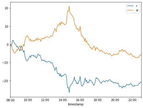
df['direction'] = 1
df.loc[df['MA20'].shift(1) > df['c'].shift(1), 'direction'] = -1
df['sr'] = df['direction'] * df['r']
display(df[['r', 'sr']].cumsum())
df[['r', 'sr']].cumsum().plot(figsize=(8,6));
| r | sr | |
|---|---|---|
| timestamp | ||
| 2021-03-30 08:00:00 | -0.49 | -0.49 |
| 2021-03-30 08:05:00 | -1.01 | 0.03 |
| 2021-03-30 08:10:00 | 0.00 | -0.98 |
| 2021-03-30 08:15:00 | 2.22 | -3.20 |
| 2021-03-30 08:20:00 | 2.24 | -3.18 |
| … | … | … |
| 2021-03-30 22:40:00 | -22.42 | -7.42 |
| 2021-03-30 22:45:00 | -21.46 | -6.46 |
| 2021-03-30 22:50:00 | -21.45 | -6.45 |
| 2021-03-30 22:55:00 | -20.79 | -5.79 |
| 2021-03-30 23:00:00 | -20.57 | -5.57 |
181 rows × 2 columns

We have defined trade direction to be 1 and if precious price is below previous candle’s MA(20) we define direction to be equal to -1 (we want to be short at that time). Then we defined strategy result (sr column) to be direction multiplied by result.
Looks pretty good? You must be aware that for vectorized test we have simplified matter pretty much. Now we will validate it even further.
Event based backtest
Previously we did vectorized backtest, which is pretty good if you want to quickly validate idea. What we saw there seemed promising, so we want to check that in more real-life conditions.
“How are we going to do that?” I hear you ask. Dear reader, in real life our program will know only price updates when they happen, which means we should implement backtest in a way that we only supply one price at the time. Let’s define it as followsIn [9]:
import math

def event_backtest(data, comm=0.0, window=20):
    close_prices = data['c']
    balances = [0]
    commission = comm # we may want to add commissions for each trade
    known_prices = []
    direction = None # at start we don't trade


    for i in range(0, len(close_prices)): # we will iterate close prices
        price = close_prices.iloc[i]
        known_prices.append(price) # remember the price, for moving average calculations

        if direction:
            balances.append(direction * (known_prices[-1] - known_prices[-2]))

        sma = pd.Series(known_prices).rolling(window).mean().iloc[-1] # calculate current MA

        if not math.isnan(sma):
            new_direction = 1 if sma < price else -1 # calculate new direction
            if new_direction != direction:
                balances[-1] = balances[-1] - commission # if direction changes we change our position, so commission apply
            direction = new_direction

    return balances
Let’s run it with commission of 1 dollar each time we do transaction:In [10]:
balances = event_backtest(df_orig, comm=1)

results = df[['r', 'sr']].copy()
results['sr-commissions'] = balances
results.cumsum().plot(figsize=(8,6));

As you can see, it’s no longer looking good – transaction costs destroyed our strategy. Unfortunately you need to find another idea, but with the knowledge from that article you will know what to do.
As you can see python data science stack is really useful when researching trading ideas. In the end, it is also working with data.

